Data science journey to highland Daghestan

This is a report on research project conducted in Linguistic Convergence Laboratory by Michael Daniel, Alexey Koshevoy, Nina Dobrushina and myself. Data and code are available on GitHub.

In statistics, we usually believe that all data points are generated as independent samples from some distribution (the well-known i.i.d. assumption). Reality is much more complex, and the following scenario is typical in applied research: we have several sources of data that represent the same underlying process but collected in a slighly different ways. Can we make sure that these differences in the data collection procedures do not introduce differences in the resulting distributions that can lead to biases in the analysis? This is the problem we faced studying traditional multilingualism in highland Daghestan, the region of Russia known for its linguistic diversity.

Reaching the past in sociolinguistic studies

More than 40 languages are spoken in Daghestan and even people in neighboring villages may have different native languages despite of strong economic and social ties between them. Thus people have to know several languages to communicate with their neighbours. These language repertoirs and their dynamics are studied by sociolinguists who are intersted which languages people spoke in the past and how their language inventory changed over time. Due to the lack of written sources, the most of the data available on this matter is collected in interviews with local people conducted during fieldtrips. Linguistic Convergence Laboratory systematically organizes such fieldtrips to collect data on multilingualism in Daghestan.

As the researchers are especially interested in the past, in these interviews respondends were asked not only about languages they speak, but also about languages their elder — often deceased — relatives spoke. This method, known as retrospective family interviews, proposed by Nina Dobrushina, allows to collect more data and reach deeper past, but also introduces a problem: how reliable the indirect data based on memories is, compared to the direct data that is obtained by asking people about themselves?

Unfortunately, we do not have time machine and cannot ask question to persons who passed away and then compare their answers with the answers we collected about them indirectly. How can we approach this problem with data science?

Comparing distributions

Instead of comparing the answers of particular respondends, we can compare the distributions of answers in direct and indirect data.

In our study, one datapoint corresponds to one person, and the variables describe this person’s socio-demographic characteristics (year of birth, gender, place of residence, etc) and a set of languages he or she speaks that is encoded as a binary vector. We also include data type variable that indicate how this datapoint was collected: is it direct or indirect data. What we are interested in is the difference between the distributions of our data depending on the value of data type variable.

Of course, we cannot expect that all variables are independent from data type. For example, year of birth and data type are clearly correlated: information from older respondents more likely to be obtained indirectly. What we can expect, instead, is that the distribution of language repertoirs of a person with given socio-demographic characteristics does not depend on the data type. If true, it means that indirect data is as much reliable as indirect one. Otherwise, we conclude that data collection through retrospective family interviews introduces biases that should be appropriately adjusted for in the analysis.

Mathematically speaking, we want to check the conditional independence between language repertoire and data type given all socio-demographic variables:

$$ (\text{language repertoire} \perp\!\!\!\perp \text{data type}) \mid \text{soc-dem}. $$

To test this hypothesis, we have to estimate the corresponding conditional (or joint) distributions from the data. This can be problematic due to high-dimensional nature of language repertoir variable. Instead, we focus on two aggregated features derived from language repertoir: knowledge of Russian (as it became lingua franca in the region since 1920’s) and index of traditional multilinguialism (ITM), that is defined as a number of languages spoken except the native language and Russian. Moreover, in the present research we limit ourselves only to the expected values of the corresponding distributions: this simplification allows us to use methods of supervised learning.

Estimating means

Machine learning models trained in supervised learning paradigm are trying to predict the value of some random variable for given values of other variables. It is well-known that with squared error loss the best possible prediction is the expected value of the corresponding conditional distribution. This suggests the following approach.

For each target variable (knowledge of Russian or ITM) we train two ML models to predict this variable using socio-demographic characteristics of a respondent. One model is trained only on direct data and the other only on indirect one. Then for each combination of socio-demographic characteristics the difference between two predictions is an estimate of the difference between expected values of the corresponding conditional distributions. And this is the difference we are interested in!

We tried several popular ML algorithms (logistic and linear regressions, random forest, gradient boosting) and decided to keep gradient boosting: it unsurprisingly demonstrated the best prediction quality on cross-validation.

Let’s look at the predictions we obtained. All results are averaged over all soc-dem variables except of year of birth.

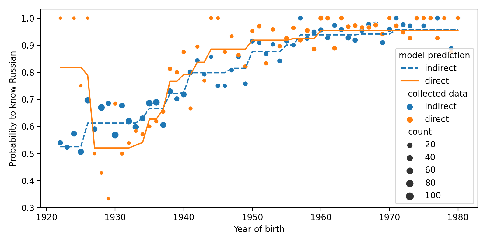
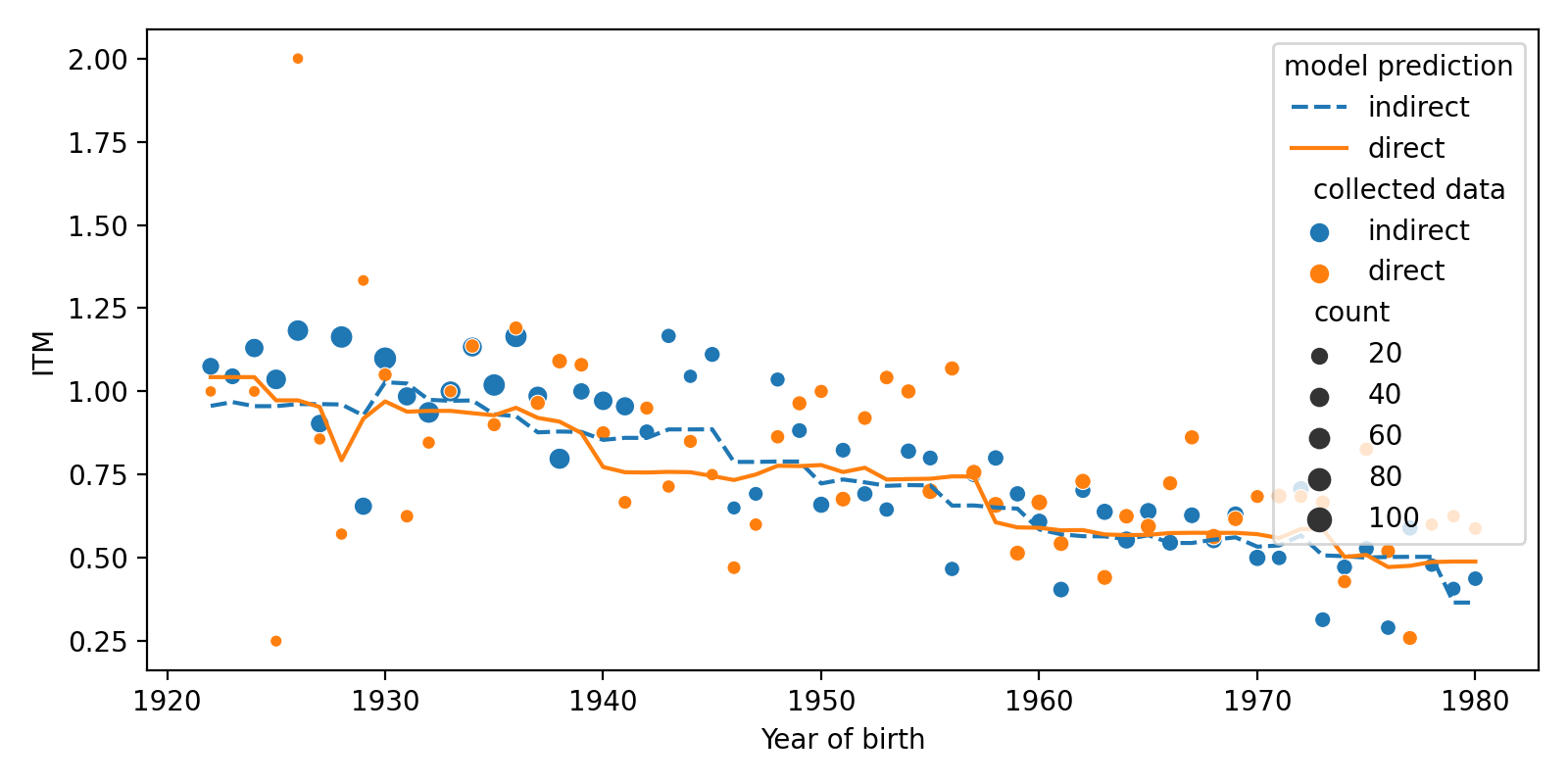
On the pictures above, we see that two lines that correspond to predictions of models trained on direct and indirect data lie close to each other, but do not coincide perfectly. How can we interpret it?

Statistics comes into play

In a perfect world, if there were no difference between direct and indirect data distributions and our models would adequately estimate the expected value of the target variable, the difference between predictions would be zero for all possible combinations of socio-demographic variables. Of course, in reality, there will be some non-zero difference due to sampling and modelling errors. Is it possible to attribute the difference we observe only to these errors? This is exactly the question of statistical hypothesis testing!

Basically, we have to test null hypothesis that there are no difference between direct and indirect data. To do it, we have to compare the results we actually observed with the results that we would observe provided that null hypothesis holds. The latter can be done by shuffling: we rearrange values in data type column randomly thus removing any statistical dependence between data type and other variables, including language repertoir. We repeat shuffling thousand times and obtain thousand new datasets, then apply our estimation procedure (i.e. train two ML models, get their predictions and find the difference between them) to these datasets. The result is a null distribution: it shows how large the difference we could possibly obtain provided that null hypothesis holds. If actually observed difference is an outlier with respect to this distribution, we can reject null hypothesis and conclude that direct and indirect data are different. Otherwise, we can attribute the observed difference to the sampling error.

Results of this analysis are shown below. On the vertical axis there is a difference between predictions of ML models trained on direct and indirect data. (For Russian, logit transformation is applied.) Red line is the difference obtained for the real data. The shaded band is an area between 2.5% and 97.5% quantiles of the null distribution (i.e. difference obtained for shuffled data) for a particular year of birth.

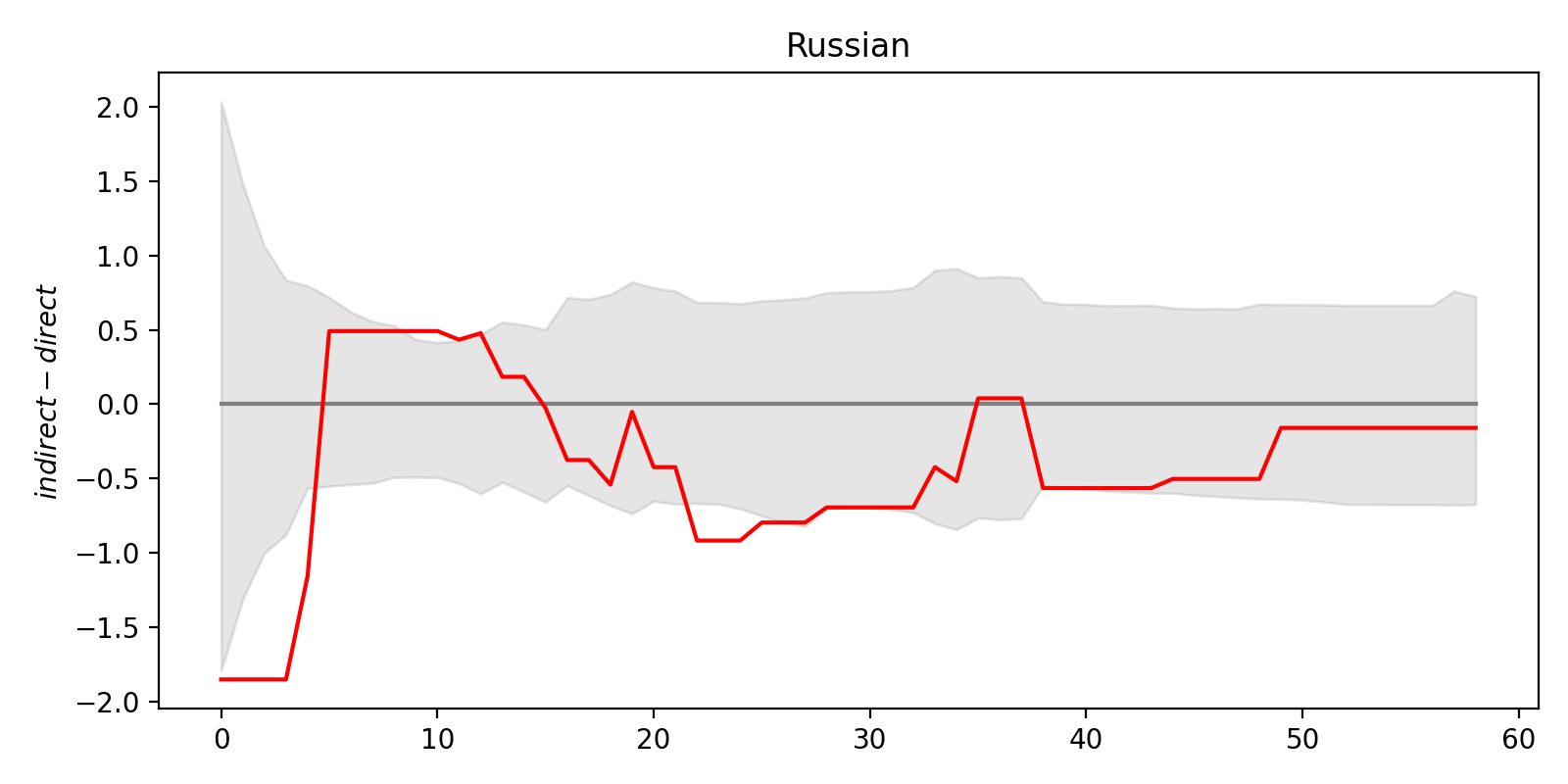
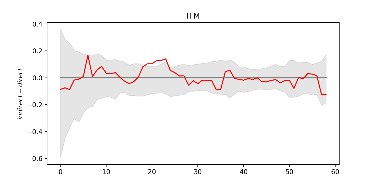
As one can see, the red lines wiggles around zero level and most of the time stays inside the shaded band. This suggests that the difference between direct and indirect data we observe may be attributed to sample error, i.e. it’s statistically insignificant. However, one have to be careful here: statistical hypothesis testing with complex objects like functions or curves can be tricky.

Testing the difference

To make sure we are on the safe side, let’s state our null hypothesis (i.e. “there are no difference between direct and indirect data”) clearly. It looks like this:

$$ H_0 \colon \ \mathbb E[y_{dir} \mid \text{soc-dem}] = \mathbb E[y_{ind} \mid \text{soc-dem}] $$ for all values of socio-demographic variables, where $y_{dir}$ and $y_{ind}$ are target variables (knowledge of Russian or ITM) for direct and indirect data respectively.

Note that we have for all clause here: if there exists at least one combination of socio-demographic variables for which expected values do not coincide, null hypothesis is false.

Let’s return to the figures above. We see that there are some points where the red line is outside of the gray band, i.e. for some years, the observed value is an outlier of the corresponding null distribution (conditional to this year). Does it mean we have to reject null hypothesis?

In fact, no. If we interpret these graphs pointwise we effectively do multiple tests: one test per each year. Thus we a prone to multiple comparison problem: as the number of tests increases, probability to make type I mistake increases as well.

On the other hand, if we would obtain a graph where the red line lies inside the shaded region, it does not automatically mean that null hypothesis shouldn’t be rejected. For example, if all values of the difference are positive, it can be considered as a strong evidence against null hypothesis no matter how small they are. Indeed, assume that the values of the difference are independent at each year, and the null hypothesis holds. In this case there are equal chances that for a particular year the difference would be negative or positive. Then it is highly unlikely to obtain a result for which all values of difference are positive.

Thus it is difficult to make accurate statistical conclusions from the figures shown above. What can we do instead?

Aggregated effect size

To overcome the issue of multiple tests, one have to consider not the whole graph of observed difference (red line on the figures), but some aggregate numeric value that shows how far it from zero value. This aggregate value can be chosen in different ways and we consider two of them.

1. Average of the difference over all possible values of the socio-demographic variables.
2. Average of the absolute value of the difference over all possible values of the socio-demographic variables.

The first value detects systematic bias, i.e. the case where the target variable is e.g. systematically larger for direct data compared with indirect data. However, it is possible that there is difference between direct and indirect data, but for different values of socio-demographic variables this difference has different signs, and they compensate each other. In this case average difference can be close to zero, but average absolute difference can be large. That’s why we consider second way to aggregate data (we call it cumulative error).

And here is the results:

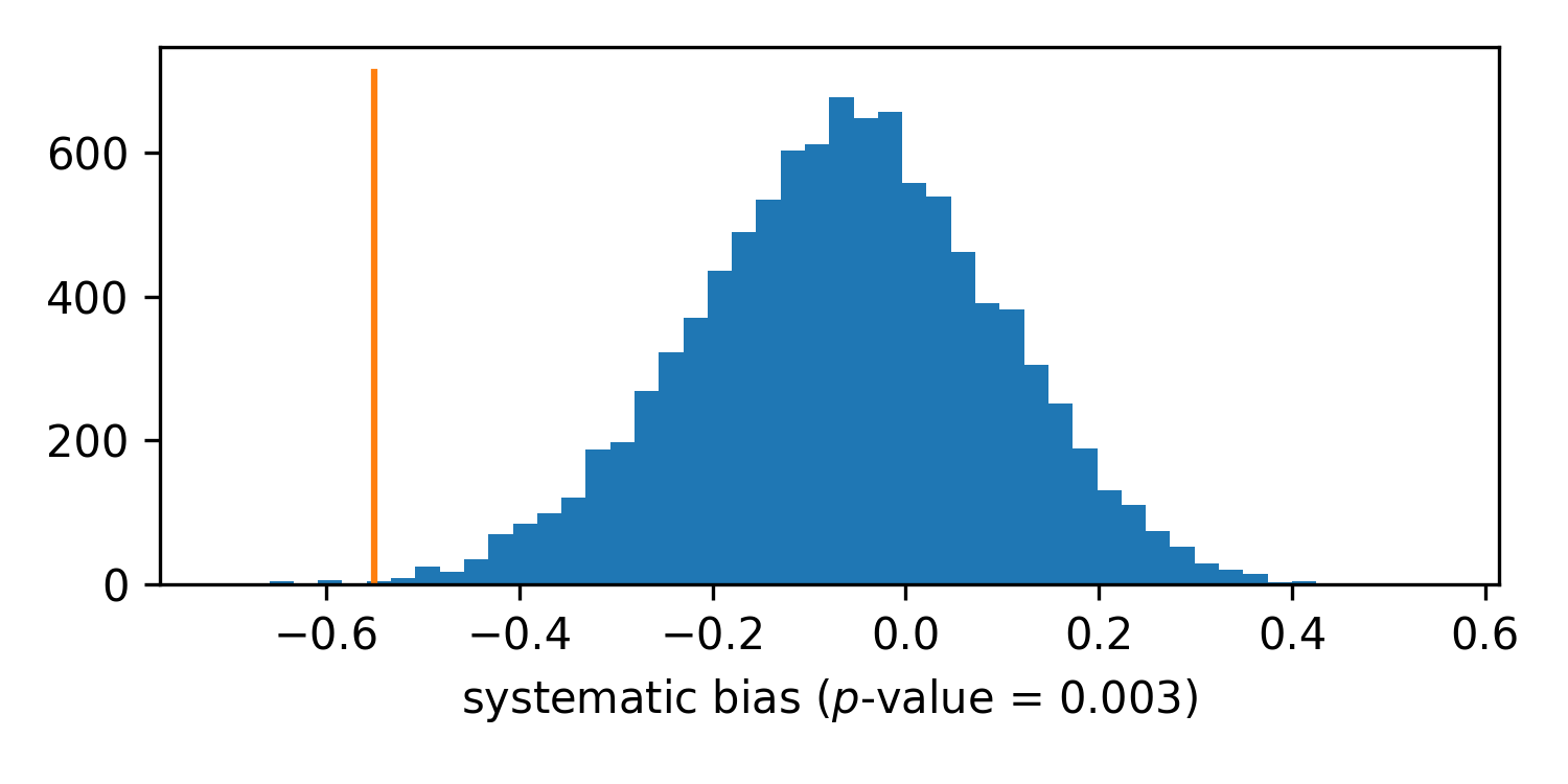
For knowledge of Russian, we see that systematic bias is detected by our test: the difference is clearly an outlier of the null distribution. It is also negative, that means that in indirect data probability to know Russian is slighly smaller than in direct data. (The average difference of logits is about 0.4.) It is in agreement with the figures above: most of the time the red line for Russian is below zero. No need to test cumulative error, as bias is already detected.

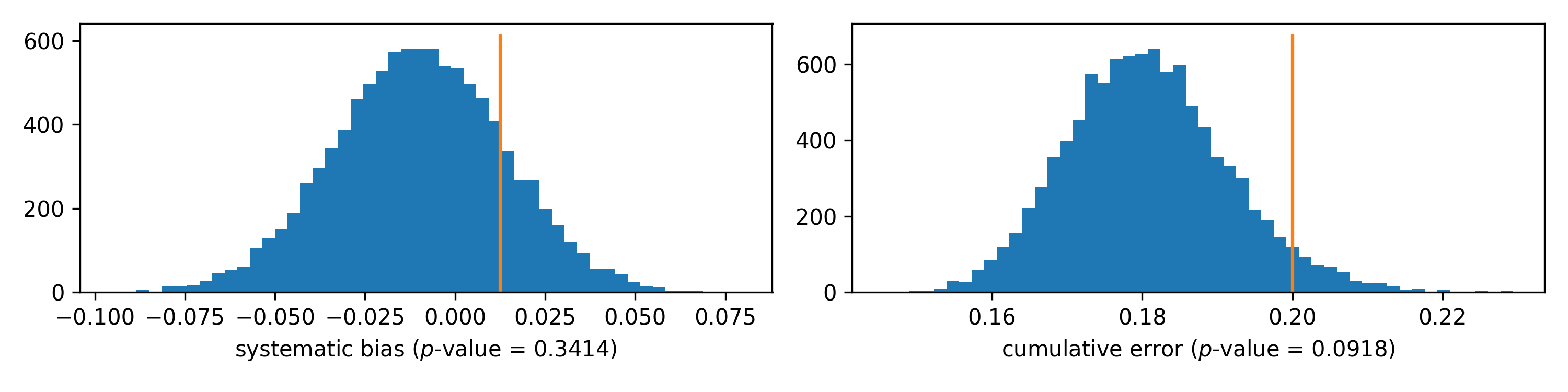
For ITM, we see neither systematic bias nor even significant cumulative error that can be detected by our methods. Of course, it doesn’t mean that we proved null hypothesis to be true: it is possible that some difference exists, but it is too small to be detectable with our data.

To understand how precise our estimates of the bias, one can construct confidence intervals. To do so, we have to estimate the standard deviation of our estimates. That can be done with bootstrap: we generate new datasets from the original one by random sampling with replacement. With this method, we obtain 95% confidence interval on systematic bias in ITM: it’s (-0.05, 0.04). Thus we can suggest that the actual value of bias, if it exists, is rather small.

Back to regressions

The method we applied in this research uses sophisticated machine learning algorithms like gradient boosting, and it can be instructive to discuss how it relates to some classical approaches.

In econometrics, when we are intersted in the effect of some variable (in our case, data type) on some other variable (e.g. knoweledge of Russian or ITM) while controlling for possible confounders (in our case, socio-demographic variables), we use linear of logistic regression — the method, known as adjustement. To simplify things, let’s consider ITM and linear regression. It looks like the following:

$$ \begin{align} \text{ITM} = \beta_0 & + \beta_1 \cdot [\text{data_type} = {\tt indirect}] \\ & + \beta_2 \cdot \text{year_of_birth} \\ & + \beta_3 \cdot [\text{gender} = {\tt female}] + \ldots \end{align} $$

Linear model assumes that the effect of data type variable (i.e. the bias we want to estimate) does not depend on the values of other variables and size of this effect is given by the corresponding coefficient ($\beta_1$ in the formula above). This effect size can be also expressed as a difference between the predictions made for direct and indirect data, similar to our approach. Due to linearity, this difference does not depend on the values of other variables, making it unnecessary to do additional steps discussed in section Testing the difference above.

These assumptions simplifies the analysis drastically: for example, regression model can learn on the whole dataset (no need to split into direct and indirect data), and the result can be interpreted straightforwardly.

Our approach is similar in nature and can be considered as a generalization of this classical adjustement procedure to non-linear machine learning models. It allows one to take into account non-linear relationships, categorical features with high cardinalities (like place of residence in our data), and dependence of the effect size on other variables, like it is shown on figures above. At the same time, with shuffling and bootstrap procedures, we can obtain rigorous statistical conclusions, similar to the results of significance testing for regression coefficients.

What’s next

At the beginning of ML course I usually discuss with students the difference between econometrics (or other classical branches of statistics) and machine learning. In my view, the main difference is our objective: in econometrics, we are interested in the model interpretation and causal effects while in machine learning we are trying to obtain the model with best predictive performance, no matter how it works. This allows to apply more complex and flexible models but reduces our abilities to use them as a scientific tool.

However, reality is non-linear in its nature, and this fact poses an intriguing and exciting problem: how can we adapt non-linear ML algorithms and techniques to use them in various scientific settings?

Our project is a step in this direction. More will follow.